
Kaggle TensorFlow Speech Recognition Challenge: Training Deep Neural Network for Voice Recognition
In this report, I will introduce my work for our Deep Learning final project. Our project is to finish the Kaggle Tensorflow Speech Recognition Challenge, where we need to predict the pronounced word from the recorded 1-second audio clips. To learn more about my work on this project, please visit my GitHub project page here.
In our first research stage, we will turn each WAV file into MFCC vector of the same dimension (the files are of the same length). In the first few hidden layers (of either multi-layer perceptron or 1-D convolutional neural net), we plan to turn the MFCC vectors into log probability of phonemes, i.e. the basic building blocks of a pronounced word. We then plan to feed these sequences to a recurrent neural network (either a RNN or a more advanced LSTM) to train and predict the word. The assumption of this approach is that the MFCC values of a sound clip should reflect the nuance sequence in word pronunciation and the the sequence is strictly ordered. Therefore, the sequence should be be used in recurrent neural networks to classify the words.
In our second research stage, we will turn each WAV file into a visual graph (called spectrogram) of the same size. Since the graphical representation of the voice has pixel points of the same scale on two dimensions, we will then apply convolutional layers on the graphs to extract latent graphical patterns from the files. We will then build fully connected layers to link the extracted feature maps to the expected output. It is even possible to feed the extracted features as a sequence to a recurrent layer since the graphical patterns should also be strictly related to time series, but the model might be too complicated for the simple task we are dealing with. The assumption of this approach is that the graphical patterns in the spectrograms of different words pronounced in the WAV files should be typical enough for the convolutional neural network to train on.
STAGE 1: Proof-of-concept training for MFCC-phonemes approach
STAGE 1.1: Pre-training an MLP for MFCC-phonemes layers
In our first stage, I will pre-train a model that can give a somewhat accurate probability estimation on phonemes based on MFCC values. The pre-training stage will help improve the complete model’s performance since the weights of corresponding layers are not randomly initiated. My first stab of this problem is a simple-structured MLP:
MLP (
  (l1): Linear (num_inputs -> 50)
  (t1): Tanh ()
  (l2): Linear (50 -> 38)
  (t2): LogSoftmax ()
)
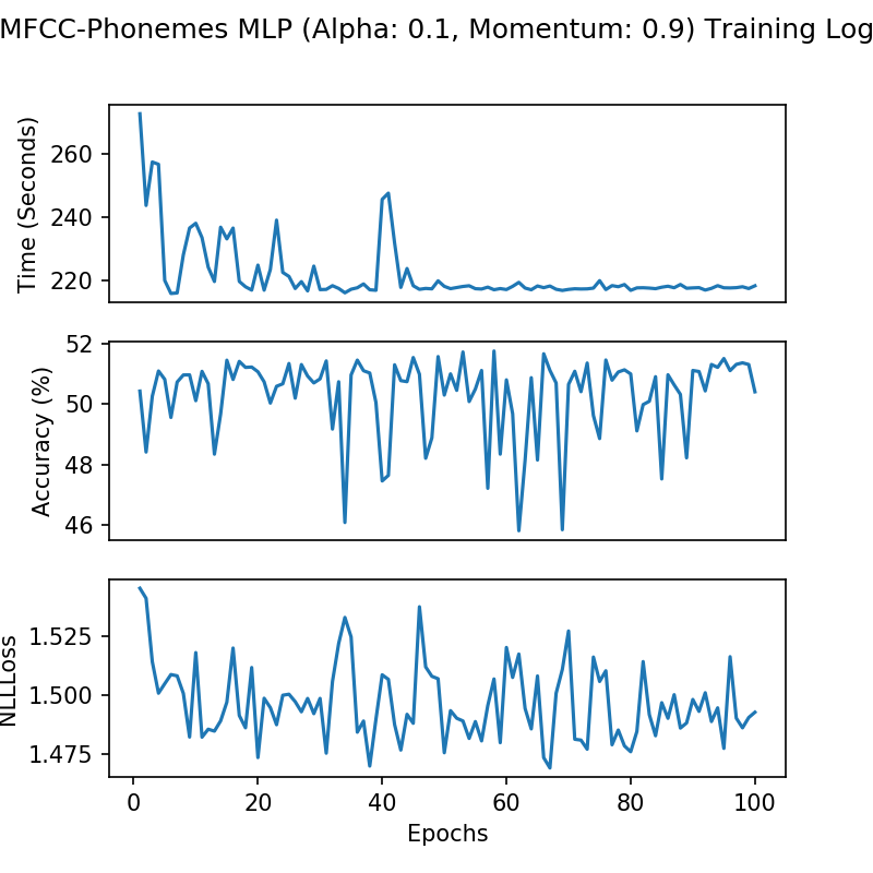
The num_inputs value is determined by our feature generation stage when the MFCC scores of the same length are calculated for each WAV file. The target phonemes have 38 possible labels. With a learning rate of 0.1 and a momentum of 0.9 for the Stochastic Gradient Descent optimization algorithm, I created a model with 51.75% accuracy. This performance is quite impressive for such a simple model, considering the natural probability of the classification being correct is only 1/38, i.e. 2.63%. The training logs of the first 100 epochs is displayed below:
STAGE 1.2: Pre-training a CNN for MFCC-phonemes layers
As an alternative to the MLP training, I also built a multi-layer convolutional neural network with 1-D kernels for each MFCC vector inputs to see if I can pre-train a better model than the MLP. Since the 39 features of MFCC vectors contain MFCC scores, deltas, and delta-deltas, I restructured the input tensor to 3 by 13, where 3 is the number of channels. By restructuring input tensors in this way, I can ensure that the three types of data are updated separately in the back propagation process. The CNN network has a structure as below:
class CNN(nn.Module):
    def __init__(self, num_inputs, num_channels):
        super(CNN, self).__init__()
        self.num_channels = num_channels
        self.feature_length = int(num_inputs / num_channels)
        self.conv1 = nn.Conv1d(num_channels, 24, 4)
        self.conv2 = nn.Conv1d(24, 48, 3)
        self.conv3 = nn.Conv1d(48, 96, 3)
        self.pool = nn.MaxPool1d(2, 2)
        self.fc1 = nn.Linear(96, 256)
        # 96 is calculated based on 13 features per channel
        self.fc2 = nn.Linear(256, 38)
        self.drop = nn.Dropout(p=0.25)
        self.t1 = nn.ReLU()
        self.t2 = nn.LogSoftmax()

    def forward(self, x):
        x = x.view(-1, self.num_channels, self.feature_length)
        x = self.t1(self.conv1(x))  # feature length 10
        x = self.t1(self.conv2(x))  # feature length 8
        x = self.drop(self.pool(x))  # feature length 4
        x = self.t1(self.conv3(x))  # feature length 2
        x = self.drop(self.pool(x))  # feature length 1, fc1 input is 1*96=96
        x = x.view(-1, 1 * 96)  # flatten feature maps to 1D
        x = self.t1(self.fc1(x))
        x = self.t2(self.fc2(x))
        return x
I also included pooling layers and dropout layers to ensure that the model do not overfit. The training logs of the first 50 epochs is displayed below:
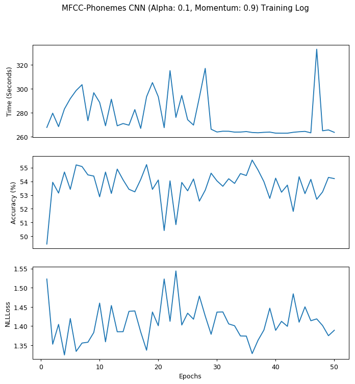
The model reached the highest accuracy at 55.55% at epoch 35.
STAGE 1.3: Concluding the MFCC-phonemes approach
The suboptimal result from the primary testing with MFCC and phonemes indicates that this traditional method is not the ideal approach that we should follow using neural network. I then seek to generate an easier network with our second approach.
STAGE 2: Training a CNN for spectrogram-word predictions
STAGE 2.1: Generating spectrograms from .WAV files
In order to train a convolutional network on graphical representation of .WAV files, I will need to preprocess the files. I used scipy package to generate the spectrograms in PNG format and generated a map file that includes the path of the PNG files and their corresponding labels. The core functions I used in this stage are as below:
def log_specgram(audio, sample_rate, window_size=20, step_size=10, eps=1e-10):
    nperseg = int(round(window_size * sample_rate / 1e3))
    noverlap = int(round(step_size * sample_rate / 1e3))
    freqs, _, spec = signal.spectrogram(audio,
                                        fs=sample_rate,
                                        window='hann',
                                        nperseg=nperseg,
                                        noverlap=noverlap,
                                        detrend=False)
    return freqs, np.log(spec.T.astype(np.float32) + eps)

def wav2img(wav_path, targetdir='', figsize=(4, 4)):
    """
    takes in wave file path
    and the fig size. Default 4,4 will make images 288 x 288
    """
    fig = plt.figure(figsize=figsize)
    samplerate, test_sound = wavfile.read(wav_path)
    _, spectrogram = log_specgram(test_sound, samplerate)
    output_file = wav_path.split('/')[-1].split('.wav')[0]
    output_file = targetdir + '/' + output_file
    plt.imsave('%s.png' % output_file, spectrogram)
    plt.close()
    return (output_file + '.png')
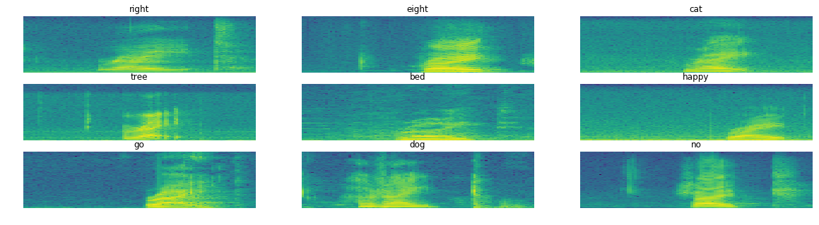
The generated spectrograms are as below:

From these samples, I have seen that different words’ spectrograms do look differently. I am hopeful that we can train a convolutional network on these inputs! The other key part of my next training stage is the map file. The generated map file has contents as below:
                                              path target
0  ../data/train/audio/right/988e2f9a_nohash_0.wav  right
1  ../data/train/audio/right/1eddce1d_nohash_3.wav  right
2  ../data/train/audio/right/93ec8b84_nohash_0.wav  right
3  ../data/train/audio/right/6272b231_nohash_1.wav  right
4  ../data/train/audio/right/439c84f4_nohash_1.wav  right
I will use the path and the target from this map file in my PyTorch stochastic mini batch training paradigm in the following stages.
STAGE 2.2: Building initial CNN for spectrogram pictures and labels
In my training script, I customized pytorch package’s handy DataSet class and DataLoader class to achieve multi-CPU fast loading and easy GPU integration. The main script for the CNN training consists of the following steps:
- Define hyper parameters for epochs, GPU usage, CPU usage, and optimization
- Load map file and define label index to replace labels with numbers
- Conduct train test split on map file
- Define spectrogram dataset and spectrogram PNG file transform methods so that PNG files and targets are automatically loaded and preprocessed into tensors of the same shape (batch_size * 3 * 99 * 161 and batch_size * 1)
- Create training and validating dataset and dataloader, where mini-batches are automatically generated using multiple CPUs
- Define CNN network structure, loss/criterion function, and optimization algorithm
- Define training, validating, and testing functions
- Write epoch loops with training, validation, and log recording
The core part of the script, i.e. the CNN network framework, is defined as below:
class CNN(nn.Module):
    def __init__(self):
        super(CNN, self).__init__()
        self.conv1 = nn.Conv2d(3, 24, 4)
        self.conv2 = nn.Conv2d(24, 48, 3)
        self.conv3 = nn.Conv2d(48, 96, 4)
        self.pool = nn.MaxPool2d(2, 2)
        self.fc1 = nn.Linear(10 * 18 * 96, 256)
        self.fc2 = nn.Linear(256, 11)
        self.drop = nn.Dropout(p=0.25)
        self.pad = nn.ZeroPad2d((0, 1, 0, 0))
        self.t1 = nn.ReLU()
        self.t2 = nn.LogSoftmax()

    def forward(self, x):
        x = self.t1(self.conv1(x))  # feature shape 96 * 158
        x = self.drop(self.pool(x))  # feature shape 48 * 79
        x = self.t1(self.conv2(x))  # feature shape 46 * 77
        x = self.drop(self.pool(self.pad(x)))  # feature shape 23 * 39
        x = self.t1(self.conv3(x))  # feature shape 20 * 36
        x = self.drop(self.pool(x))  # feature shape 10 * 18
        x = x.view(-1, 10 * 18 * 96)  # flatten feature maps to 1D
        x = self.t1(self.fc1(x))
        x = self.t2(self.fc2(x))
        return x
Be noted that the model takes three layers of kernels to reduce the input size to reasonably-sized 10 by 18 feature maps before being fed to fully connected layers for prediction. The script takes num_workers and use_gpu parameters that define number of CPUs for batch loading and whether to use GPUs for model training, separately. I ran the model on an instance on the Google Cloud Platform with 1 GPU and 10 CPUs; training the model locally with no GPUs is likely to take too much time to finish.
STAGE 2.3: Fine tuning model with class weight and optimization hyper parameters
It is worth noting that the project only needs 11 tags for the output prediction, while the training input has more than 30 word tags. I had to relabel most of the word tags into “unknown” to match the desired output. However, after I relabeled the target by replacing non-voice-command words with a single label “unknown”, I observed an unbalanced dataset where samples with the “unknown” label is 17.44 times the size of other samples. When trained with this unbalanced data, I noticed that the trained CNN model will simply label all samples with the ‘unknown’ label to achieve the “best” NLLLoss score, such as below:
# first row is the prediction for 'unknown'
Confusion Matrix:
[[4080    0    0    0    0    0    0    0    0    0    0]
 [ 248    0    0    0    0    0    0    0    0    0    0]
 [ 264    0    0    0    0    0    0    0    0    0    0]
 [ 238    0    0    0    0    0    0    0    0    0    0]
 [ 219    0    0    0    0    0    0    0    0    0    0]
 [ 243    0    0    0    0    0    0    0    0    0    0]
 [ 230    0    0    0    0    0    0    0    0    0    0]
 [ 239    0    0    0    0    0    0    0    0    0    0]
 [ 225    0    0    0    0    0    0    0    0    0    0]
 [ 256    0    0    0    0    0    0    0    0    0    0]
 [ 231    0    0    0    0    0    0    0    0    0    0]]
To deal with the unbalanced data in the training set, I therefore implemented a class weight to penalize the predictions for ‘unknown’ class so that all labels have an equal weight regardless of the sample size. Hence my weight tensor is defined as label_weight = torch.FloatTensor([0.057, 1, 1, 1, 1, 1, 1, 1, 1, 1, 1]), where 0.057 equals 1/17.44. After adjusting for the class weights, I received the following confusion matrix early in the training epochs with a NLLoss of 0.41:
Confusion Matrix:
[[1516 1358  203  111   95   58  497  104   22   22   94]
 [   1  230    6    2    5    1    1    0    2    0    0]
 [   1   96   95    1   63    2    6    0    0    0    0]
 [   5   18    3  175   13    2    5    2    0    2   13]
 [   2   78   18    1  116    1    2    0    0    0    1]
 [   2    9    9    2    0  140   69    0    0   12    0]
 [   2   15    2    1    0    3  204    2    1    0    0]
 [  28    9    8   13    0    0    5  175    0    0    1]
 [   4   50   11    2    0    7    6    0  137    8    0]
 [   4   19   22    3    2   33   30    1    4  138    0]
 [   5   13    1    3    2    0    2    2    0    0  203]]
This looks much like what a confusion matrix is ‘supposed’ to be like: the model is actually learning from the input data now that the target is better defined. I then proceeded to hyper-parameter tuning, starting with a 5-epoch run with the standard learning rate at 0.1 and momentum at 0.9, as shown below:
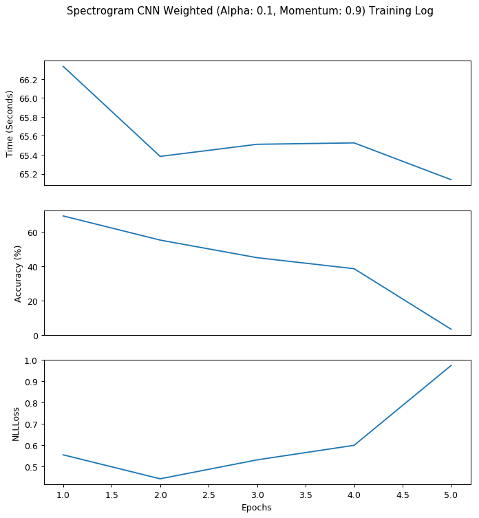
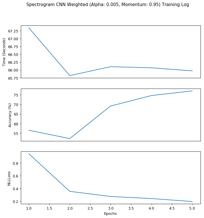
We can see from this chart that the model overshot the global minimum after epoch 2 since the NLLLoss is steadily increasing afterwards. I will need to adjust the hyper-parameter to make the model learn much more slowly. Therefore, in my second 5-epoch run I defined learning rate as 0.005 and momentum as 0.95; my result is displayed below:
With a smaller gradient descent step and a larger jump over local minimums, we can clearly see that the model is learning steadily from the input data this time: the NLLLoss is steadily decreasing and the accuracy is steadily increasing. Therefore, I decided that these combination of hyper-parameter is what we desired and went forward to train the data with 30 epochs. My result is displayed below:
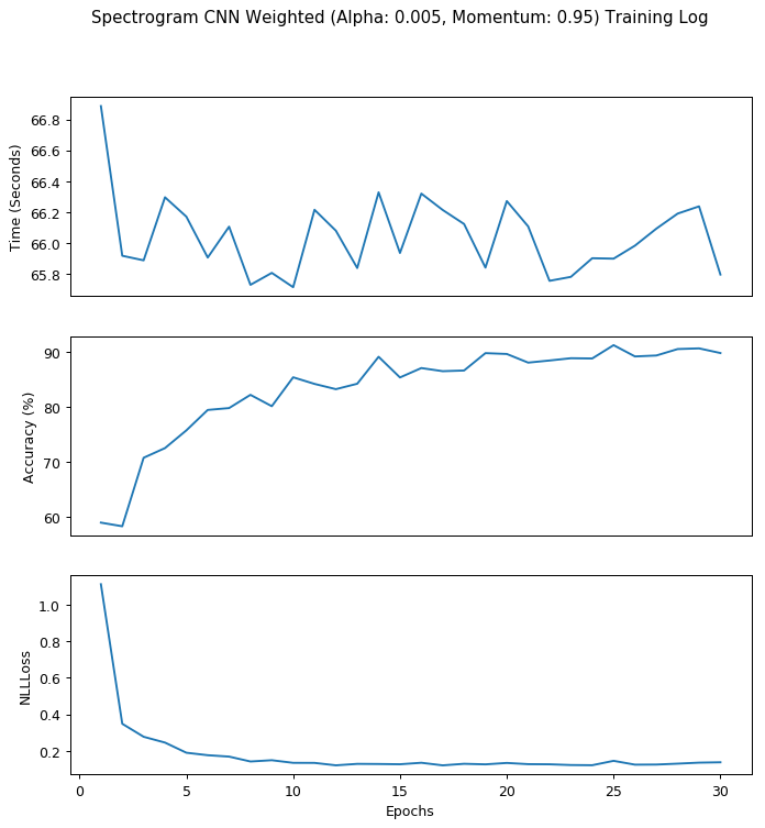
Within 30 epochs, we have our highest accuracy at epoch 25 with the confusion matrix as below:
[Epoch 25] Accuracy: 91.24%, Average Loss: 0.15
Confusion Matrix:
[[3753   30   77   11   22   38   53   56   20   12    8]
 [  13  221    9    1    1    0    1    0    2    0    0]
 [   5    7  231    2   14    0    2    1    1    1    0]
 [  19    0    0  216    0    0    0    1    0    0    2]
 [   7    6   20    1  181    0    0    1    1    2    0]
 [   8    0    1    1    1  215    6    0    1   10    0]
 [  14    0    1    0    0    2  212    0    0    1    0]
 [   8    0    1    1    1    0    0  228    0    0    0]
 [   6    2    2    1    0    4    2    1  200    7    0]
 [   6    1    2    1    0   14    1    0    4  227    0]
 [   9    0    0    0    0    0    0    0    0    0  222]]
The best average NLLLoss, however, was achieved at epoch 17 with the confusion matrix as below:
[Epoch 17] Accuracy: 86.50%, Average Loss: 0.12
Confusion Matrix:
[[3431   47   54   73   60   88   80  110   49   37   51]
 [   9  218    3    0   10    2    2    0    3    0    1]
 [   2    7  218    3   25    2    3    1    1    2    0]
 [   5    0    0  224    2    1    0    1    0    0    5]
 [   5    7   10    3  187    0    0    0    1    4    2]
 [   4    1    0    2    0  222    5    0    1    8    0]
 [   6    1    0    0    0    6  214    0    0    2    1]
 [   3    0    1    3    1    0    0  231    0    0    0]
 [   2    3    1    1    0    6    2    0  205    5    0]
 [   4    1    1    2    0   16    1    0    6  225    0]
 [   2    0    0    2    0    0    1    1    1    0  224]]


Leave a Comment