Introduction to Machine Learning with Python - Chapter 2 - Linear Models for Classification

Below is my study notes from learning the book Introduction to Machine Learning with Python. Refer to the author’s GitHub repo at https://github.com/amueller/introduction_to_ml_with_python.

import sys
print("Python version: {}".format(sys.version))
import pandas as pd
print("pandas version: {}".format(pd.__version__))
import matplotlib
print("matplotlib version: {}".format(matplotlib.__version__))
import numpy as np
print("NumPy version: {}".format(np.__version__))
import scipy as sp
print("SciPy version: {}".format(sp.__version__))
import IPython
print("IPython version: {}".format(IPython.__version__))
import sklearn
print("scikit-learn version: {}".format(sklearn.__version__))
import mglearn
print("mglearn version: {}".format(mglearn.__version__))
import math
import matplotlib.pyplot as plt
from sklearn.model_selection import train_test_split

%matplotlib inline

Python version: 3.6.0 |Continuum Analytics, Inc.| (default, Dec 23 2016, 12:22:00)
[GCC 4.4.7 20120313 (Red Hat 4.4.7-1)]
pandas version: 0.19.2
matplotlib version: 1.5.3
NumPy version: 1.11.3
SciPy version: 0.18.1
IPython version: 5.1.0
scikit-learn version: 0.18.1
mglearn version: 0.1.3

1.6 Linear Models for Classification

In the case of Linear Models for classification, the predicted value threshold is set at zero (i.e. a logical determination of whether the target values meet the conditions or not).

Let’s look at binary classification first. In this case, a prediction is made using the following formula: ŷ = w[0] * x[0] + w[1] * x[1] + … + w[p] * x[p] + b > 0

The above formula, when reflected on chart, will appear to be a decision boundary that seperates two categoreis using a line, a plane, or a hyperplane.

1.6.1 Common Models for Linear Classification

All algorithms for linear classification models differ in the following two ways:

• How models measure how well a particular combination of coefficients and intercept fits the training data
• If any, what kind of regularization they use

Two most commen linear classification algorithms:

• Logistic Regression: linear_model.LogisticRegression
• Linear Support Vector Machines: svm.LinearSVC (Support Vector Classifier)

Let’s see how these two algorithms apply on the forge dataset.

from sklearn.linear_model import LogisticRegression
from sklearn.svm import LinearSVC
X, y = mglearn.datasets.make_forge()
fig, axes = plt.subplots(1, 2, figsize=(10, 3))
for model, ax in zip([LinearSVC(), LogisticRegression()], axes):
    clf = model.fit(X, y)
    mglearn.plots.plot_2d_separator(clf, X, fill=False, eps=0.5,
    ax=ax, alpha=.7)
    mglearn.discrete_scatter(X[:, 0], X[:, 1], y, ax=ax)
    ax.set_title("{}".format(clf.__class__.__name__))
    ax.set_xlabel("Feature 0")
    ax.set_ylabel("Feature 1")
axes[0].legend()

<matplotlib.legend.Legend at 0x7fbc0be314a8>

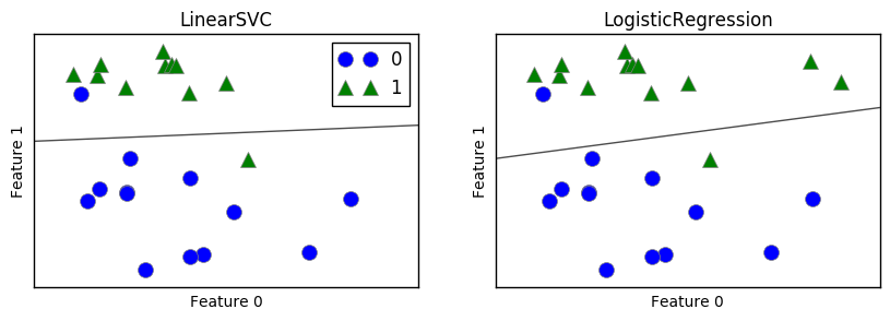
In the above graphs, the line is the decision boundary that would determine the category of dots falling above or under the line. If the points fall above the line, they would be categorized as Category 1 and under as Category 0.

1.6.1.1 Tweaking the regularization parameters for LogisticRegression and LinearSVC

By default, both models apply an L2 regularization, in the same way that Ridge does for regression.

For LogisticRegression and LinearSVC the trade-off parameter that determines the strength of the regularization is called C, and higher values of C correspond to less regularization. In other words, when you use a high value for the parameter C, LogisticRegression and LinearSVC try to fit the training set as best as possible, while with low values of the parameter C, the models put more emphasis on finding a coefficient vector (w) that is close to zero.

Using low values of C will cause the algorithms to try to adjust to the “majority” of data points, while using a higher value of C stresses the importance that each individual data point be classified correctly.

mglearn.plots.plot_linear_svc_regularization()

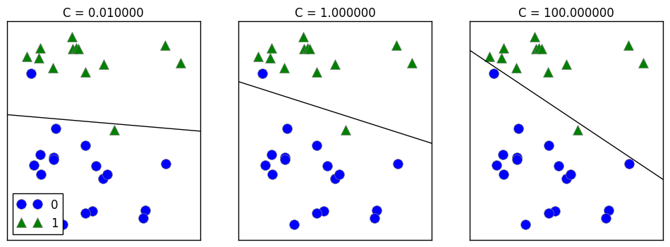
On the left, the strongly regularized model choose a relatively horizontal line by following only the general trend: that category 1 points are above and category 0 points are below.

On the right, since the regularization is been set to really low, the line tries its best to correctly categorize the points. Therefore, all points in category 0 is been identified.

The right option might overfit since it is trying over hard to fit ALL OF THE POINTS in the test set.

1.6.2 Logistic Regression

1.6.2.1 LinearLogistic on Breast Cancer dataset

from sklearn.datasets import load_breast_cancer
cancer = load_breast_cancer()
X_train, X_test, y_train, y_test = train_test_split(
cancer.data, cancer.target, stratify=cancer.target, random_state=42)
logreg = LogisticRegression().fit(X_train, y_train)
print("Training set score: {:.3f}".format(logreg.score(X_train, y_train)))
print("Test set score: {:.3f}".format(logreg.score(X_test, y_test)))

Training set score: 0.955
Test set score: 0.958

The default value for C in LogisticRegression is 1. However, since the training and test sets have close scores, it is likely that the model is underfitting. Let’s try a more flexible model setting.

logreg100 = LogisticRegression(C=100).fit(X_train, y_train)

print("Training set score: {:.3f}".format(logreg100.score(X_train, y_train)))
print("Test set score: {:.3f}".format(logreg100.score(X_test, y_test)))

Training set score: 0.972
Test set score: 0.965

The more flexible (i.e. more complex) model have better performance in both training and test set. Just to compare the models, we can try a even more restricted model with C = 0.01.

logreg001 = LogisticRegression(C=0.01).fit(X_train, y_train)

print("Training set score: {:.3f}".format(logreg001.score(X_train, y_train)))
print("Test set score: {:.3f}".format(logreg001.score(X_test, y_test)))

Training set score: 0.934
Test set score: 0.930

As expected, more restricted model results in lower performance and closer accuracy for both training and testing set. It’s time for us to examine again the performance-complexity graph.

training_accuracy = []
test_accuracy = []

# try C from 0.00001 to 1000
C_settings = [0.0001, 0.001, 0.01, 0.05, 0.1, 0.5, 1, 3, 5, 7, 10, 20, 30, 50, 70, 100]

for C in C_settings:
    # build the model
    logreg = LogisticRegression(C=C)
    logreg.fit(X_train, y_train)
    # record training accuracy
    training_accuracy.append(logreg.score(X_train, y_train))
    # record generalization accuracy
    test_accuracy.append(logreg.score(X_test, y_test))

plt.plot(np.array(C_settings),
         training_accuracy, label="training accuracy")
plt.plot(np.array(C_settings),
        test_accuracy, label="test accuracy")
plt.ylabel("Accuracy")
plt.xlabel("C logs")
plt.legend(loc=4)

<matplotlib.legend.Legend at 0x7fbc093981d0>

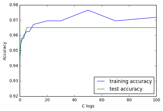
As we can expect from the C settings, having more and more flexible model makes the training accuracy more and more accurate; however, the accuracy of the data on the test set hits a plateau at around C = 5.

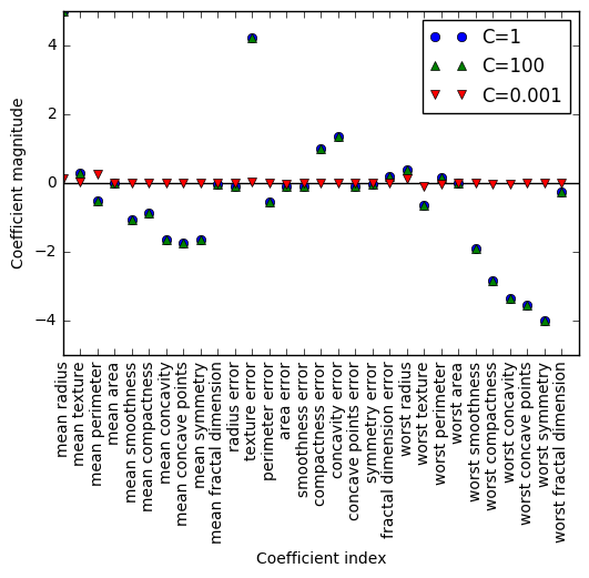
Finally, let’s check out the coefficient combinations of the models at different levels of C.

plt.plot(logreg.coef_.T, 'o', label="C=1")
plt.plot(logreg100.coef_.T, '^', label="C=100")
plt.plot(logreg001.coef_.T, 'v', label="C=0.001")
plt.xticks(range(cancer.data.shape[1]), cancer.feature_names, rotation=90)
plt.hlines(0, 0, cancer.data.shape[1])
plt.ylim(-5, 5)
plt.xlabel("Coefficient index")
plt.ylabel("Coefficient magnitude")
plt.legend()

<matplotlib.legend.Legend at 0x7fbc09314f28>