Introduction to Machine Learning with Python - Chapter 2 - Linear Models for Continuous Target

Below is my study notes from learning the book Introduction to Machine Learning with Python. Refer to the author’s GitHub repo at https://github.com/amueller/introduction_to_ml_with_python.

import sys
print("Python version: {}".format(sys.version))
import pandas as pd
print("pandas version: {}".format(pd.__version__))
import matplotlib
print("matplotlib version: {}".format(matplotlib.__version__))
import numpy as np
print("NumPy version: {}".format(np.__version__))
import scipy as sp
print("SciPy version: {}".format(sp.__version__))
import IPython
print("IPython version: {}".format(IPython.__version__))
import sklearn
print("scikit-learn version: {}".format(sklearn.__version__))
import mglearn
print("mglearn version: {}".format(mglearn.__version__))
import math
import matplotlib.pyplot as plt
from sklearn.model_selection import train_test_split

%matplotlib inline

Python version: 3.6.0 |Continuum Analytics, Inc.| (default, Dec 23 2016, 12:22:00)
[GCC 4.4.7 20120313 (Red Hat 4.4.7-1)]
pandas version: 0.19.2
matplotlib version: 1.5.3
NumPy version: 1.11.3
SciPy version: 0.18.1
IPython version: 5.1.0
scikit-learn version: 0.18.1
mglearn version: 0.1.3

1.5 Linear Models for Regression

For regression, the general prediction formula for a linear model looks as follows:

ŷ = w[0] * x[0] + w[1] * x[1] + … + w[p] * x[p] + b

Here, x[0] to x[p] denotes the features (in this example, the number of features is p) of a single data point, w and b are parameters of the model that are learned, and ŷ is the prediction the model makes. For a dataset with a single feature, this is:

ŷ = w[0] * x[0] + b

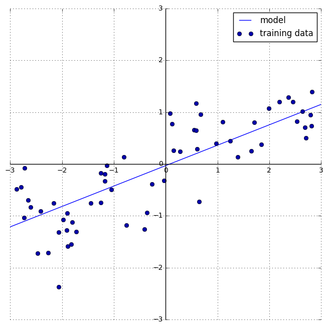
For Linear Regression models, the bigger the absolute values of the coefficients, the more complex the model is. In other words, the flatter the linear line, the simpler the model is.

mglearn.plots.plot_linear_regression_wave()

w[0]: 0.393906  b: -0.031804

Definition of Linear Models

Linear models for regression can be characterized as regression models for which the prediction is a line for a single feature, a plane when using two features, or a hyperplane in higher dimensions (that is, when using more features).

Linear models can be extra powerful for a wide dataset, i.e. dataset with more features than training data points. We can start by learning the most popular regression model.

1.5.1 Lenear regression (aka ordinary least squares, OLS)

Linear regression finds the parameters w and b that minimize the mean squared error between predictions and the true regression targets, y, on the training set.

Features of OLS

• No parameters
• Cannot control model complexity

from sklearn.linear_model import LinearRegression
X, y = mglearn.datasets.make_wave(n_samples = 60)
X_train, X_test, y_train, y_test = train_test_split(X, y, random_state=42)

lr = LinearRegression().fit(X_train, y_train)

The fitted OLS model has two parameters, as below:

print("lr.coef_: {}".format(lr.coef_))
print("lr.intercept_: {}".format(lr.intercept_))

# parameters generated from the training data will have "_" at the
# tail, whereas parameters set by users don't

lr.coef_: [ 0.39390555]
lr.intercept_: -0.03180434302675973

The model’s performance on training set and test set is as below:

print("Training set score: {:.2f}".format(lr.score(X_train, y_train)))
print("Test set score: {:.2f}".format(lr.score(X_test, y_test)))

Training set score: 0.67
Test set score: 0.66

The linear regression’s performance on a simple dataset is not really impressive. But we will now test it on a complex Boston Housing dataset.

1.5.1.1 OLS on Boston Housing dataset

X, y = mglearn.datasets.load_extended_boston()
X_train, X_test, y_train, y_test = train_test_split(X, y, random_state=0)
lr = LinearRegression().fit(X_train, y_train)

print("Training set score: {:.2f}".format(lr.score(X_train, y_train)))
print("Test set score: {:.2f}".format(lr.score(X_test, y_test)))

Training set score: 0.95
Test set score: 0.61

Since OLS does not give options to control complexity, this model is overfitting. We will then look at an alternative to OLS, which is Ridge Regression.

1.5.2 Ridge Regression

Ridge Regression is the basic OLS model plus the following restriction:

We also want the magnitude of coefficients to be as small as possible; in other words, all entries of w should be close to zero. Intuitively, this means each feature should have as little effect on the outcome as possible (which translates to having a small slope), while still predicting well.

This process, called L2 regularization helps to explicitly avoid overfitting.

The sklearn uses Ridge class to instantiate Ridge Regressions.

from sklearn.linear_model import Ridge

ridge = Ridge().fit(X_train, y_train)

print("Training set score: {:.2f}".format(ridge.score(X_train, y_train)))
print("Test set score: {:.2f}".format(ridge.score(X_test, y_test)))

Training set score: 0.89
Test set score: 0.75

The default parameter for Ridge model is alpha = 1.0. By changing the alpha value when instantiating the class, users can adjust the level of restrictions on the Ridge Regression.

Higher Alpha -> Stronger restriction -> Parameter magnitude closer to zero

ridge10 = Ridge(alpha=10).fit(X_train, y_train)
print("Training set score: {:.2f}".format(ridge10.score(X_train, y_train)))
print("Test set score: {:.2f}".format(ridge10.score(X_test, y_test)))

ridge01 = Ridge(alpha=0.1).fit(X_train, y_train)
print("\nTraining set score: {:.2f}".format(ridge01.score(X_train, y_train)))
print("Test set score: {:.2f}".format(ridge01.score(X_test, y_test)))

Training set score: 0.79
Test set score: 0.64

Training set score: 0.93
Test set score: 0.77

X, y = mglearn.datasets.load_extended_boston()
X_train, X_test, y_train, y_test = train_test_split(X, y, random_state=0)
lr = LinearRegression().fit(X_train, y_train)

training_accuracy = []
test_accuracy = []

# try alpha from 0.01 to 10
alpha_settings = [0.01, 0.05, 0.1, 0.2, 0.3, 0.4, 0.5, 0.6, 0.7, 0.8, 0.9, 1.0, 2.0, 3.0, 4.0, 5.0, 6.0, 7.0, 8.0, 9.0, 10.0]

for alpha in alpha_settings:
    # build the model
    ridge = Ridge(alpha=alpha)
    ridge.fit(X_train, y_train)
    # record training accuracy
    training_accuracy.append(ridge.score(X_train, y_train))
    # record generalization accuracy
    test_accuracy.append(ridge.score(X_test, y_test))

plt.plot(np.log(np.array(alpha_settings)),
         training_accuracy, label="training accuracy")
plt.plot(np.log(np.array(alpha_settings)),
        test_accuracy, label="test accuracy")
plt.ylabel("Accuracy")
plt.xlabel("alpha logs")
plt.legend()

<matplotlib.legend.Legend at 0x7fd00d0c76d8>

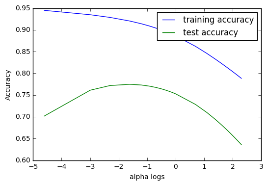
As we can see from above graph, the performance of Ridge Regression model on the test set hits the highest point when the natural logarithm of the alpha is between -2 and -1. Considering the decreasing nature of the training accuracy, we should prefer an alpha within this range that is as low as possible.

print("log alpha array: {}".
      format(np.around(np.log(np.array(alpha_settings)),3)))
print("alpha array: {}".format(np.array(alpha_settings)))

print("Training performance: {:.5f}".format(training_accuracy[3]))
print("Test performance: {:.5f}".format(test_accuracy[3]))

log alpha array: [-4.605 -2.996 -2.303 -1.609 -1.204 -0.916 -0.693 -0.511 -0.357 -0.223
 -0.105  0.     0.693  1.099  1.386  1.609  1.792  1.946  2.079  2.197
  2.303]
alpha array: [  0.01   0.05   0.1    0.2    0.3    0.4    0.5    0.6    0.7    0.8    0.9
   1.     2.     3.     4.     5.     6.     7.     8.     9.    10.  ]
Training performance: 0.92028
Test performance: 0.77468

From the alpha arrays, we observe that the fourth alpha meets our conditions; i.e. when alpha = 0.2, we will see the optimized Ridge Model.

1.5.2.1 Under the Hood for Ridge Regressions

We can also get a more qualitative insight into how the alpha parameter changes the model by inspecting the coef_ attribute of models with different values of alpha. A higher alpha means a more restricted model, so we expect the entries of coef_ to have smaller magnitude for a high value of alpha than for a low value of alpha.

plt.plot(ridge.coef_, 's', label="Ridge alpha=1")
plt.plot(ridge10.coef_, '^', label="Ridge alpha=10")
plt.plot(ridge01.coef_, 'v', label="Ridge alpha=0.1")
plt.plot(lr.coef_, 'o', label="LinearRegression")
plt.xlabel("Coefficient index")
plt.ylabel("Coefficient magnitude")
plt.hlines(0, 0, len(lr.coef_))
plt.ylim(-25, 25)
plt.legend()

<matplotlib.legend.Legend at 0x7fd00d019eb8>

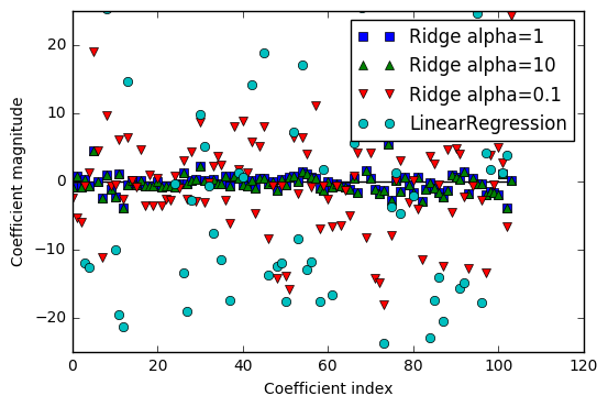
From above graph we can see that with alpha larger, the coefficients are most condensed near the w=0 line.

Learning Curves

Another way to understand the influence of regularization is to fix a value of alpha but vary the amount of training data available.

we subsampled the Boston Housing dataset and evaluated LinearRegression and Ridge(alpha=1) on subsets of increasing size (plots that show model performance as a function of dataset size are called learning curves)

mglearn.plots.plot_ridge_n_samples()

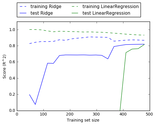
Because ridge is regularized, the training score of ridge is lower than the training score for linear regression across the board. However, the test score for ridge is better, particularly for small subsets of the data. For less than 400 data points, linear regression is not able to learn anything. As more and more data becomes available to the model, both models improve, and linear regression catches up with ridge in the end.

Key Takeaway

With enough training data, regularization becomes less important, and given enough data, ridge and linear regression will have the same performance.

1.5.3 Lasso Regression

Lasso Regression uses L1 Regualtion to regularize the regression.

The consequence of L1 regularization is that when using the lasso, some coefficients are exactly zero. This means some features are entirely ignored by the model. This can be seen as a form of automatic feature selection. Having some coefficients be exactly zero often makes a model easier to interpret, and can reveal the most important features of your model.

from sklearn.linear_model import Lasso

lasso = Lasso().fit(X_train, y_train)

print("Training set score: {:.2f}".format(lasso.score(X_train, y_train)))
print("Test set score: {:.2f}".format(lasso.score(X_test, y_test)))
print("Number of features used: {}".format(np.sum(lasso.coef_ != 0)))

Training set score: 0.29
Test set score: 0.21
Number of features used: 4

Apparently the default setting for this lasso regression is underfitting on the Houston Housing dataset.

Similarly, Lasso Regression also has alpha = 1.0 as its parameter. The larger alpha is, the simpler the model is.

Another parameter, max_iter (maximum number of iterations to run) should also be defined. The smaller alpha is, the larger max_iter should be.

# We increase the default setting of max_iter
# And decrease alpha
lasso001 = Lasso(alpha=0.01, max_iter=100000).fit(X_train, y_train)

print("Training set score: {:.2f}".format(lasso001.score(X_train, y_train)))
print("Test set score: {:.2f}".format(lasso001.score(X_test, y_test)))
print("Number of features used: {}".format(np.sum(lasso001.coef_ != 0)))

Training set score: 0.90
Test set score: 0.77
Number of features used: 33

The adjusted model ended up using 33 out of the 105 features in the dataset. This makes it potentially easier to understand.

If we set alpha too low, the model will become too complicated and more similar to OLS.

lasso00001 = Lasso(alpha=0.0001, max_iter=100000).fit(X_train, y_train)
print("Training set score: {:.2f}".format(lasso00001.score(X_train, y_train)))
print("Test set score: {:.2f}".format(lasso00001.score(X_test, y_test)))
print("Number of features used: {}".format(np.sum(lasso00001.coef_ != 0)))

Training set score: 0.95
Test set score: 0.64
Number of features used: 94

training_accuracy = []
test_accuracy = []

# try alpha from 0.00001 to 10
alpha_settings = [0.00001, 0.0001, 0.001, 0.01, 0.05, 0.1, 0.5, 1, 2, 4, 8, 10]

for alpha in alpha_settings:
    # build the model
    lasso = Lasso(alpha=alpha, max_iter=10000000)
    lasso.fit(X_train, y_train)
    # record training accuracy
    training_accuracy.append(lasso.score(X_train, y_train))
    # record generalization accuracy
    test_accuracy.append(lasso.score(X_test, y_test))

plt.plot(np.log(np.array(alpha_settings)),
         training_accuracy, label="training accuracy")
plt.plot(np.log(np.array(alpha_settings)),
        test_accuracy, label="test accuracy")
plt.ylabel("Accuracy")
plt.xlabel("alpha logs")
plt.legend()

<matplotlib.legend.Legend at 0x7fd00cf92860>

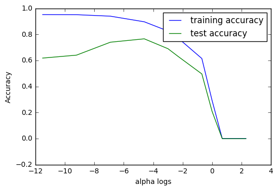
Similarly to the redge regression, the “sweet spot” for this specific case comes at -6 < log(alpha) < -4. We can check it out by looking at the corresponding arrays.

print("log alpha array: {}".
      format(np.around(np.log(np.array(alpha_settings)),3)))
print("alpha array: {}".format(np.array(alpha_settings)))

print("Sweet spot alpha: {}".format(alpha_settings[3]))
print("Training performance: {:.5f}".format(training_accuracy[3]))
print("Test performance: {:.5f}".format(test_accuracy[3]))

log alpha array: [-11.513  -9.21   -6.908  -4.605  -2.996  -2.303  -0.693   0.      0.693
   1.386   2.079   2.303]
alpha array: [  1.00000000e-05   1.00000000e-04   1.00000000e-03   1.00000000e-02
   5.00000000e-02   1.00000000e-01   5.00000000e-01   1.00000000e+00
   2.00000000e+00   4.00000000e+00   8.00000000e+00   1.00000000e+01]
Sweet spot alpha: 0.01
Training performance: 0.89651
Test performance: 0.76565

1.5.3.1 Under the Hood for Lasso Regressions

plt.plot(lasso.coef_, 's', label="Lasso alpha=1")
plt.plot(lasso001.coef_, '^', label="Lasso alpha=0.01")
plt.plot(lasso00001.coef_, 'v', label="Lasso alpha=0.0001")
plt.plot(ridge01.coef_, 'o', label="Ridge alpha=0.1")
plt.legend(ncol=2, loc=(0, 1.05))
plt.ylim(-25, 25)
plt.xlabel("Coefficient index")
plt.ylabel("Coefficient magnitude")

<matplotlib.text.Text at 0x7fd00ce0b2e8>

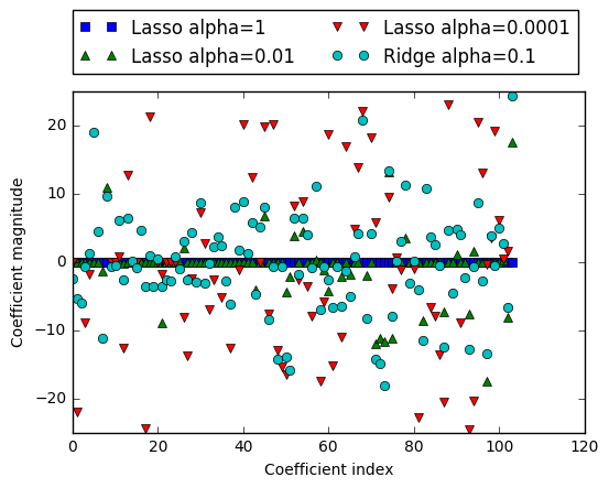
In practice, ridge regression is usually the first choice between these two models.

However, if you have a large amount of features and expect only a few of them to be important, Lasso might be a better choice. Similarly, if you would like to have a model that is easy to interpret, Lasso will provide a model that is easier to understand, as it will select only a subset of the input features.